Understanding SISO Systems and Control Theory in Practice

Key takeaways from this article:

• SISO systems with one input and output find diverse applications, from industrial automation to consumer electronics, driven by linear equations and transfer functions.
• Transfer functions decode system behavior, stability analysis techniques ensure robustness and feedback control mechanisms regulate SISO systems effectively.
• In radio technology, SISO setups’ simplicity contrasts MIMO’s resilience against interference, a vital consideration for optimal performance.

In this article, we’ll break down what SISO systems are all about, and why it’s a fundamental concept that forms one of the cornerstones of control theory. As engineers, we’re always looking for ways to make things faster and more reliable, why you’ll want to have this concept under your skin.

Single-Input Single-Output

A SISO system is a configuration centered around a variable, featuring a single input and a corresponding output. It’s a scenario where a single control signal influences a single response. SISO systems are often used to model and control linear time-invariant systems, where the behavior doesn’t change over time and can be described by linear equations.

There are three essential methods for SISO system control: transfer functions, stability analysis, and feedback control:

• Transfer functions decode how a system responds to varying input frequencies using a ratio of Laplace transforms, providing insights into frequency response, stability, and performance.
• In stability analysis, engineers ensure system stability by analyzing through methods like root locus and Nyquist criterion, visualizing root movement and the frequency response’s impact on overall stability.
• Feedback loops compare system output to reference values, adjusting input for regulation. Proportional-Integral-Derivative (PID) controllers exemplify feedback control in SISO systems.

Mathematically, SISO systems are typically described using differential equations, transfer functions, or state-space representations. Differential equations provide a dynamic description of the system’s behavior in terms of rates of change, while transfer functions offer a frequency-domain perspective that simplifies analysis. State-space representations describe the system using a set of first-order differential equations, making it easier to work with modern control techniques.

We’ll talk more about the SISO system control functions later in the article.

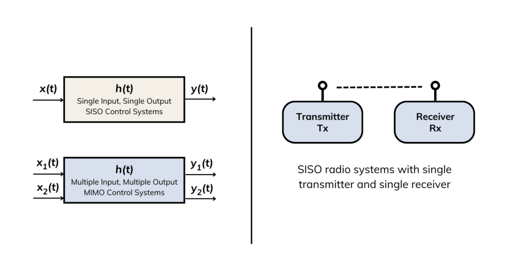
Left: SISO and MIMO control systems. Right: SISO radio system with single transmitter and receiver.

Applications of SISO Systems

In a Single-Input Single-Output system, the input can vary widely depending on the specific application, encompassing factors such as voltage, force, pressure, or temperature. Similarly, the output reflects measurable responses such as velocity, displacement, or position, which are influenced by the input. At the heart of SISO systems lies the fundamental relationship between input and output, elucidating the cause-and-effect dynamics within the system.

Some examples of SISO systems include:

With industrial automation, for example, in manufacturing plants, SISO controllers regulate variables such as temperature, pressure, or flow rate. Think about your home thermostat—it’s a classic example. The input (chosen temperature) influences the output (room temperature), and the controller adjusts the system to maintain the desired condition. In environmental control, HVAC (Heating, ventilation, and air conditioning) systems are another classic example of exactly this.

If we look at consumer electronics such as audio systems, the volume knob acts as an input, and the resulting sound level is the output. Similarly, in washing machines, the cycle settings (the input) dictate the washing intensity and duration (the output).

In biomedical engineering and medical applications, SISO systems can model and control physiological variables like blood pressure, heart rate, or drug dosage. For instance, think about an insulin pump. It keeps track of the patient’s glucose level—that’s the input—and adjusts the insulin dosage accordingly.

The list of examples is long, and of course, there are many more than just the ones we’ve mentioned. But you probably have a good idea of the SISO principle by now, and we don’t want to bore you with endless examples. The important thing is, that you understand that single input = single output.

SISO Transfer Functions

Transfer functions are a key concept of SISO control theory. They provide a concise representation of how a system responds to different frequencies of input signals. A transfer function is a ratio of the Laplace transforms of the output and input signals, often denoted as:

H(s) = Y(s)/X(s), where Y(s) and X(s) are the Laplace transforms of the output and input signals.

Transfer functions allow engineers to analyze system behavior in the frequency domain, enabling insights into frequency response, stability, and performance characteristics. They are particularly valuable for designing controllers that can shape a system’s behavior to meet specific requirements. For instance, engineers can use transfer functions to design filters that attenuate certain frequency components or controllers that ensure the system responds optimally to different inputs.

Stability Analysis

Stability is a critical concern in control systems, as an unstable system can lead to undesirable oscillations or even devastating failures. In SISO control, engineers have a couple of tricks up their sleeves to check for stability. One is the root locus method, and the other is the Nyquist criterion.

The Root Locus Method is a graphical technique that helps to visualize how a system’s poles (characteristic roots) change with different control gains. Engineers can evaluate the impact of the gain adjustments on stability and system performance by mapping the potential root locations in the complex plane.

Then there’s the Nyquist Criterion. This one’s also a graphical technique. It represents the relation of the system’s frequency response to its stability. It gives you a way to figure out if the system stats stable based on the number of encirclements of the critical point (-1) in the complex plane.

Feedback Control for SISO Systems

Feedback control is an important concept in SISO systems. In a feedback control loop, the system’s output gets measured, compared with what we want it to be, and then used to tweak the system’s input. This helps keep the system in check, aiming to reduce any gaps between the desired and actual outputs.

PID (Proportional-Integral-Derivative) controllers are a common example of feedback control. They tweak the control input according to the current error (The gap between the desired and actual outputs), how that error adds up over time, and how fast it changes. Think of it as fine-tuning a recipe to get the perfect dish. Just like adjusting the seasoning, you can tweak the PID controller’s settings to get the system to behave the way you want – whether that means getting it to settle down quickly, avoiding overshooting the mark, or just keeping things steady.

SISO for Radio Technology

In a SISO radio system, you’ve only got a single antenna each for the transmitter and the receiver, lacking multiple antenna setups. When we talk about antenna technology, it can come in different forms, either indicating single or multiple inputs and outputs, all connected by the radio link. Think of it like a game of connecting the dots but with antennas and signals.

To break it down simply, the input resembles the transmitter, and the output resembles the receiver. The transmitter sends its’ signals into the link, which is then picked up by the receiver, located at the end of the wireless path.