


Key takeaways from this article:
- Adaptive grid refinement in mesh generation significantly enhances computational efficiency by accurately resolving both geometry and physics.
- The incorporation of refinement zones based on simulation expectations, as illustrated in the article, showcases a proactive approach to optimizing mesh quality for specific flow features, such as those around vehicles.
- Domain expertise and user input play crucial roles in ensuring the effectiveness of adaptive grid refinement, preventing over-refinement in areas with minimal flow physics to avoid unnecessary computational costs and simulation time.
In this article, we’re going to elaborate on the automated adaptive grid refinement feature in Fidelity Pointwise. It handles numerical errors and sticks to boundaries set by the user while accurately resolving all flow features for various applications.
Simulation preprocessing aims to create a mesh that fits the required analysis. You should prioritize computational efficiency in generating a mesh that accurately captures both geometry and physics. Depending on your simulation objectives, you can refine specific areas of the mesh where smaller flow features are expected.
In the illustration below, refinement zones have been incorporated around the vehicle to account for anticipated physics, particularly in the wake region. This process requires substantial domain expertise and relies on user input. Excessive refinement in regions with minimal flow physics would unnecessarily increase computation costs and simulation time, which is not what you would want.
Mesh adaptation: what are the requirements?
When creating a mesh it should fulfill the following requirements:
- Align with the underlying CAD geometry
- Honor locally anisotropic boundary layer refinement
- Enhance both significant and subtle flow features
In adaptive grid refinement, preservation of the boundary layer and near-wall physics is anticipated, alongside a gradual transition in cell sizes to ensure solver convergence. Defining an adaptation sensor is essential during grid refinement, outlining areas needing further enhancement. For external aircraft analyses, the Mach number serves as a suitable adaptation variable, whereas in turbomachinery scenarios, velocity magnitude proves effective as an adaptation sensor.
Adaptive grid refinement using Fidelity Pointwise
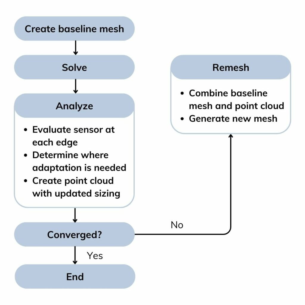
First off, we lay down a baseline mesh to kickstart the adaptive grid refinement in Fidelity Pointwise. Then, a solution is run on this mesh. You would want to evaluate the sensor at each edge. If it goes over your predetermined threshold at any spot, you’ll raise the adaptation flag. Next up, a point cloud is created, pinpointing locations, and setting a fresh cell size for the area. This cloud gets merged into the baseline mesh within Fidelity Pointwise to create an updated mesh. Rinse and repeat this process until your solution stands tall on its own, independent of the mesh.
Application test cases
Impinging Jet
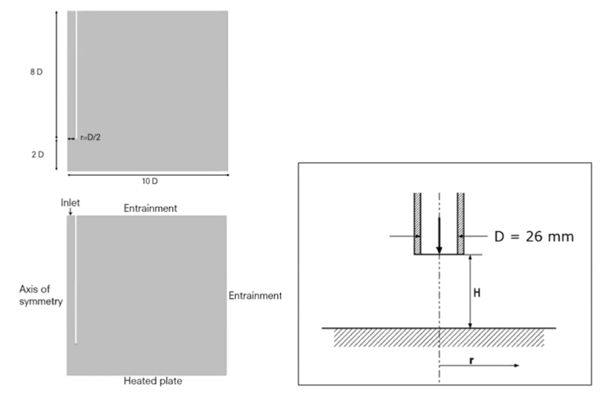
In the figure above, we’ve got a cold jet swooping down onto a hot plate, with all the boundary conditions laid out for you.
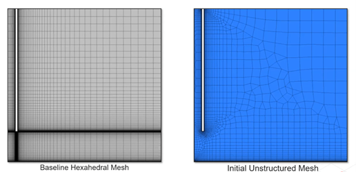
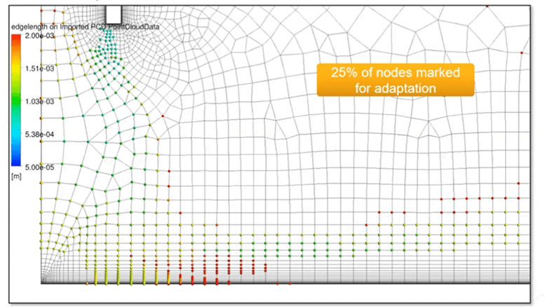
The goal here is to do a side-by-side comparison of a fully structured mesh versus an adapted one. On the left, you’ve got the baseline hexahedron mesh, while on the right, you’ve got the initial unstructured mesh, ready to adapt to the velocity magnitude.
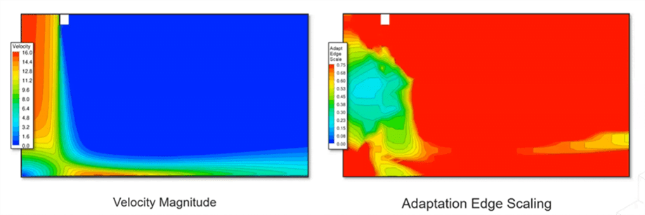
We’ve highlighted the scaling needed for the current edge lane in the image on the right. The adaptation process zeroes in on the area sandwiched between the jet and the plate. We’ve created a point cloud from the solution, and about a quarter of the nodes have hit the threshold and are due for some tweaking.
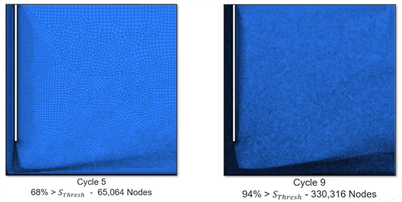
By the fifth cycle, roughly 70% of the nodes were flagged for adaptation, with a whopping 94% getting the mark by the final cycle. Once we hit around 90% adaptation, we call it quits on the iterations.
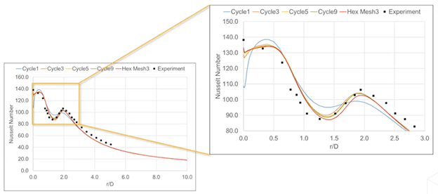
Looking at the mesh stats, it’s clear that the tweaked mesh boasts fewer nodes and elements compared to the meticulously crafted hex mesh. Zooming into the impingement region reveals that the initial mesh missed the mark, but with each cycle, it got closer to the experimental data.
Axial turbine blade
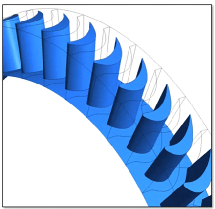
Alright, buckle up! In this scenario, we’re testing out an Aachen Turbine (as seen in the illustration above) with 41 blades, spinning away at a brisk 3500 RPM. Let’s check out the flow conditions at the inlet and outlet, neatly laid out in the table below:
| P total (inlet) | 169,000 Pa |
| T total (inlet | 308 K |
| A (inlet) | 49.3° |
| P outlet | 135,000 Pa (average) |
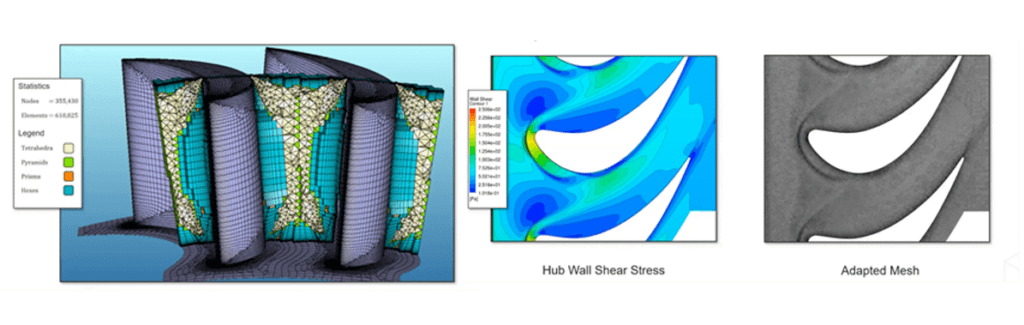
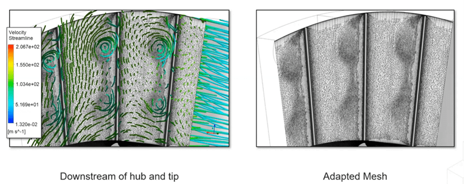
And again, we’re keeping an eye on the velocity magnitude for our adaptation variable. Those shockwaves are front and center in our adapted mesh. Plus, look at the final adapted mesh—it’s spot-on in showcasing those secondary vortices and shocks.
DrivAer model
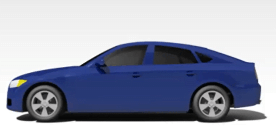
Adaptive grid refinement isn’t limited to specific applications; it’s also valuable in automotive settings. In the illustration above, we’re examining the DrivAer model. Our focus is on the velocity magnitude as the adaptation variable.
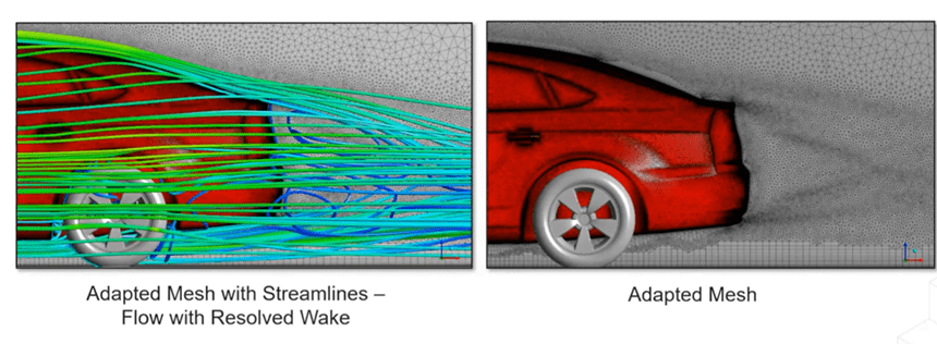
A RANS simulation of the DrivAer model employs the SST two-equation turbulence model. Below, you’ll find the adapted mesh and the streamlines in the wake region. They illustrate a strong correspondence and effectively capture the vortices.
External Aerodynamics
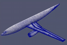
Let’s look at a DLR F6 model, a test case from the second AIAA drag prediction workshop. Flow conditions include a Mach number of 0.75 and a 1° angle of attack. We’re honing in on the Mach number as our adaptation variable here.
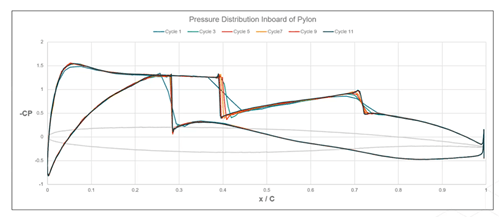
With adaptive grid refinement, those shockwaves atop the wing come into sharp focus. Check out the figure below, showcasing the initial and adapted surface pressures. The shocks get crisper with each adaptation cycle.
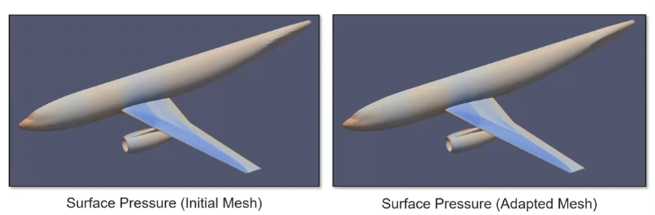
Now, when we look at the coefficient of lift and drag, it’s evident that refinement gets finer with every cycle. This mesh adaptation technique can seamlessly slot into any workflow.
While there’s a bit of legwork upfront to set things up, once established, it runs independently. The adaptation cycle consistently maintains the mesh’s topology, cycling back to the baseline.
If you want to learn more, Cadence has a free on-demand webinar on how to automatically generate the best mesh each time with adaptive grid refinement in Fidelity Pointwise. You can find it right here.